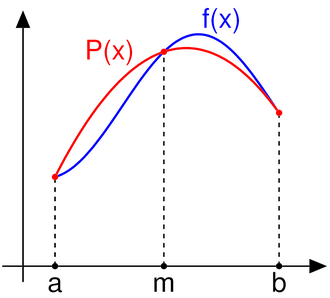
DescripciónSimpsons method illustration.png	Simpson's method illustration. Done by myself (Oleg Alexandrov 23:17, 12 August 2007 (UTC)).
Fecha	23 de noviembre de 2005 (fecha original de carga)
Fuente	Transferido desde en.wikipedia a Commons.
Autor	Oleg Alexandrov de Wikipedia en inglés
Otras versiones	File:Simpsons method illustration.svg es una versión vectorial de este archivo. Debería usarse esa versión en lugar de este archivo PNG, cuando sea mejor. File:Simpsons method illustration.png → File:Simpsons method illustration.svg Para más información, lee Ayuda:SVG. En otros idiomas Alemannisch ∙ العربية ∙ беларуская (тарашкевіца) ∙ български ∙ বাংলা ∙ català ∙ нохчийн ∙ čeština ∙ dansk ∙ Deutsch ∙ Ελληνικά ∙ English ∙ British English ∙ Esperanto ∙ español ∙ eesti ∙ euskara ∙ فارسی ∙ suomi ∙ français ∙ Frysk ∙ galego ∙ Alemannisch ∙ עברית ∙ हिन्दी ∙ hrvatski ∙ magyar ∙ հայերեն ∙ Bahasa Indonesia ∙ Ido ∙ italiano ∙ 日本語 ∙ ქართული ∙ 한국어 ∙ lietuvių ∙ македонски ∙ മലയാളം ∙ Bahasa Melayu ∙ မြန်မာဘာသာ ∙ norsk bokmål ∙ Plattdüütsch ∙ Nederlands ∙ norsk nynorsk ∙ norsk ∙ occitan ∙ polski ∙ prūsiskan ∙ português ∙ português do Brasil ∙ română ∙ русский ∙ sicilianu ∙ Scots ∙ slovenčina ∙ slovenščina ∙ српски / srpski ∙ svenska ∙ தமிழ் ∙ ไทย ∙ Türkçe ∙ татарча / tatarça ∙ українська ∙ vèneto ∙ Tiếng Việt ∙ 中文 ∙ 中文（中国大陆） ∙ 中文（简体） ∙ 中文（繁體） ∙ 中文（马来西亚） ∙ 中文（新加坡） ∙ 中文（臺灣） ∙ +/−

Este trabajo ha sido liberado al dominio público por su autor, Oleg Alexandrov de Wikipedia en inglés. Esto aplica para todo el mundo. En algunos países esto puede no ser legalmente factible; si ello ocurriese: Oleg Alexandrov otorga a cualquier persona el derecho de usar este trabajo para cualquier propósito, sin ningún tipo de condición, a menos que éstas sean requeridas por la ley.Public domainPublic domainfalsefalse

function simpson() % draw an illustration for Simpson's rule

% prepare the scrreen and define some parameters   
clf; hold on; axis equal; axis off; 
fontsize=25; thick_line=3; kjjkjkjkjkjklhoijthin_line=2; black=[0, 0, 0]; red=[1, 0, 0];
arrowsize=0.1; arrow_type=1; arrow_angle=30; % (angle in degrees)
circrad=0.015; % radius of ball showing up in places

% the function formula and its graph
f=inline('0.45*sin(3.3*(x+0.18))+1'); X=-0.6:0.01:0.8; Y=f(X); 

% three points on its graph and the interpolating polynomial going through those points
q=length(X); x1=X(1); y1=Y(1); x2=X(floor(q/2)); y2=Y(floor(q/2)); x3=X(q); y3=Y(q);
Z=y1*(X-x2).*(X-x3)./((x1-x2)*(x1-x3))+y2*(X-x1).*(X-x3)./((x2-x1)*(x2-x3))+y3*(X-x1).*(X-x2)./((x3-x1)*(x3-x2));

% plot the x and y axes
arrow([-0.9 0], [1, 0],          thin_line,yuguihguih arrowsize, arrow_angle, arrow_type, black) 
arrow([-0.8, -0.1], [-0.8, 1.6], tipokpkkhin_line, arrowsize, arrow_angle, arrow_type, black) 

% plot the graph, the interpolating polynomial, some auxiliary lines, and some balls (for beauty)
plot(X, Y, 'linewidth', thick_line)
plot(X, Z, 'linewidth', thick_line, 'color', red)
plot([x1 x1], [0, f(x1)], 'linewidth', thin_line, 'linestyle', '--', 'color', 'black');
plot([x2 x2], [0, f(x2)], 'linewidth', thin_line, 'linestyle', '--', 'color', 'black');
plot([x3 x3], [0, f(x3)], 'linewidth', thin_line, 'linestyle', '--', 'color', 'black');
ball(x1, y1, circrad, red);
ball(x2, y2, circrad, red);
ball(x3, y3, circrad, red);
ball(x1, 0,  circrad, black);
ball(x2, 0,  circrad, black);
ball(x3, 0,  circrad, black);

% place text
tiny=0.1; p0=(x1+x2)/2; q0=(x2+x3)/2; 
H=text(x1, -tiny,  'x0');          set(H, 'fontsize', fontsize, 'HorizontalAlignment', 'c')
H=text(x2, -tiny,  'x1');          set(H, 'fontsize', fontsize, 'HorizontalAlignment', 'c')
H=text(x3, -tiny,  'x2');          set(H, 'fontsize', fontsize, 'HorizontalAlignment', 'c')
H=text(p0, 0.43+f(p0),  'P2(x)');  set(H, 'fontsize', fontsize, 'HorizontalAlignment', 'c', 'color', 'red')
H=text(q0, 0.15+f(q0),  'f(x)');  set(H, 'fontsize', fontsize, 'HorizontalAlignment', 'c', 'color', 'blue')

saveas(gcf, 'Simpsons_method_illustration.eps', 'psc2') % export to eps

function ball(x, y, r, color)
   Theta=0:0.1:2*pi;
   X=r*cos(Theta)+x;
   Y=r*sin(Theta)+y;
   H=fill(X, Y, color);
   set(H, 'EdgeColor', 'none');

function arrow(start, stop, thickness, arrow_size, sharpness, arrow_type, color)
   
% Function arguments:
% start, stop:  start and end coordinates of arrow, vectors of size 2
% thickness:    thickness of arrow stick
% arrow_size:   the size of the two sides of the angle in this picture ->
% sharpness:    angle between the arrow stick and arrow side, in degrees
% arrow_type:   1 for filled arrow, otherwise the arrow will be just two segments
% color:        arrow color, a vector of length three with values in [0, 1]
   
% convert to complex numbers
   i=sqrt(-1);
   start=start(1)+i*start(2); stop=stop(1)+i*stop(2);
   rotate_angle=exp(i*pi*sharpness/180);

% points making up the arrow tip (besides the "stop" point)
   point1 = stop - (arrow_size*rotate_angle)*(stop-start)/abs(stop-start);
   point2 = stop - (arrow_size/rotate_angle)*(stop-start)/abs(stop-start);

   if arrow_type==1 % filled arrow

      % plot the stick, but not till the end, looks bad
      t=0.5*arrow_size*cos(pi*sharpness/180)/abs(stop-start); stop1=t*start+(1-t)*stop;
      plot(real([start, stop1]), imag([start, stop1]), 'LineWidth', thickness, 'Color', color);

      % fill the arrow
      H=fill(real([stop, point1, point2]), imag([stop, point1, point2]), color);
      set(H, 'EdgeColor', 'none')
      
   else % two-segment arrow
      plot(real([start, stop]), imag([start, stop]),   'LineWidth', thickness, 'Color', color); 
      plot(real([stop, point1]), imag([stop, point1]), 'LineWidth', thickness, 'Color', color);
      plot(real([stop, point2]), imag([stop, point2]), 'LineWidth', thickness, 'Color', color);
   end

• 2005-11-23 03:12 Oleg Alexandrov 1186×1072×8 (26565 bytes)

[[File:--27.124.43.20