Diferencia entre revisiones de «Dibujar un sólido 2-D»
De MateWiki
| Línea 24: | Línea 24: | ||
[[Mesh of a parametrized 2-D solid]] | [[Mesh of a parametrized 2-D solid]] | ||
| + | [[Visualization of a scalar field in a solid]] | ||
| + | [[Visualization of vector fields in a solid]] | ||
[[Categoría:Curso ICE]] | [[Categoría:Curso ICE]] | ||
[[Categoría:Teoría de Campos]] | [[Categoría:Teoría de Campos]] | ||
Revisión del 13:03 19 nov 2013
We show how to draw meshes of plane regions, representing solids, with Octave UPM. The objective is to be able of visualizing physical quantities in the mesh points. We start with the simplest example, the rectangle [math] [-1/2,1/2]\times [0,2][/math]. We follow the steps:
- We introduce a sampling of the two segments with a suitable step
- With meshgrid command we define two matrixes with the x and y coordenates of the mesh points
- We use the mesh command to draw the mesh and adjunst the axis. We see the mesh from the top.
1 MATLAB code
x=-0.5:0.1:0.5;       % sampling of the interval [-1/2,1/2]
y=0:0.1:2;            % sampling of the interval [0,2]
[xx,yy]=meshgrid(x,y); % matrixes of x and y coordinates
figure(1)
mesh(xx,yy,0*xx)       % Draw the mesh
axis([-2,2,-1,3])      % select region for drawing
view([0,0,1])          % See the pisture from the top
2 Example
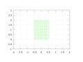
Mesh in a rectangular solid

3 To go further
Mesh of a parametrized 2-D solid Visualization of a scalar field in a solid Visualization of vector fields in a solid