Diferencia entre revisiones de «Level sets of a scalar field»

Revisión del 00:17 20 nov 2013

We show how to visualize level sets of scalar fields on plane regions with Octave UPM. We focus on the example in Dibujar un sólido 2-D, i.e. the rectangle [math] [-1/2,1/2]\times [0,2][/math] and the scalar field [math] f(x,y)=-\log (0.1+\sqrt{x^2+y^2})[/math]. We follow the steps:

1. We introduce a sampling of the two segments with a suitable step
2. With meshgrid command we define two matrixes with the x and y coordenates of the mesh points
3. Compute the scalar field in the grid points.
4. We use the contour command to draw the field and adjunst the axis. We see the picture from the top.

1 MATLAB code

x=-0.5:0.1:0.5;       % sampling of the interval [-1/2,1/2]
y=0:0.1:2;            % sampling of the interval [0,2]
[xx,yy]=meshgrid(x,y); % matrixes of x and y coordinates
figure(1)
f=-log(0.1+sqrt(xx.^2+yy.^2)); % The scalar field
contour(xx,yy,f)       % Draw the level sets
axis([-2,2,-1,3])      % select region for drawing
view(2)                % See the pisture from the top

2 Example

• 

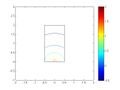
  Level sets of a scalar function