Diferencia entre revisiones de «Flujo de Poiseuille (Grupo 9B)»
(→Ecuación de Navier-Stokes para fluidos incompresibles) |
(→Caudal) |
||
| (No se muestran 87 ediciones intermedias del mismo usuario) | |||
| Línea 6: | Línea 6: | ||
Para la creación de este artículo, se ha hecho uso de programa informático Matlab para la representación gráfica de mallados, gradientes, etc. | Para la creación de este artículo, se ha hecho uso de programa informático Matlab para la representación gráfica de mallados, gradientes, etc. | ||
| − | |||
=== Mallado de la sección === | === Mallado de la sección === | ||
| Línea 30: | Línea 29: | ||
=== Ecuación de Navier-Stokes para fluidos incompresibles === | === Ecuación de Navier-Stokes para fluidos incompresibles === | ||
En física, las ecuaciones de Navier-Stokes son un conjunto de ecuaciones en derivadas parciales no lineales que describen el movimiento de un fluido viscoso. | En física, las ecuaciones de Navier-Stokes son un conjunto de ecuaciones en derivadas parciales no lineales que describen el movimiento de un fluido viscoso. | ||
| − | + | En este caso, la velocidad de las partículas del fluido viene dada por el campo vectorial <math>\overrightarrow{u}\left ( \rho ,\theta ,z \right )=f\left ( \rho \right )\overrightarrow{ez}</math> y su presión <math>p\left ( x,y \right )=p1+\left ( p2-p1 \right )\left ( z-1 \right )</math>, donde <math>\mu</math> es el coeficiente de viscosidad, p1 es la presión en los puntos z = 1, p2 la presión en los puntos z = 2. | |
| − | <math>\left ( \overrightarrow{u}\cdot \bigtriangledown \right )\cdot u +\bigtriangledown p = \mu \Delta \overrightarrow{u}</math> | + | |
| + | Se utilizará la ecuación de Navier-Stoker estacionaria (independiente del tiempo), ya que <math>\left ( \overrightarrow{u},p \right )</math> satisface dicha ecuación. Se va despreciar el primer término, la parte convectiva. | ||
| + | <math>\left ( \overrightarrow{u}\cdot \bigtriangledown \right )\cdot u +\bigtriangledown p = \mu \Delta \overrightarrow{u}</math>. | ||
| + | |||
Se comprueba que <math>f\left ( \rho \right )</math> satisface la ecuación diferencial: | Se comprueba que <math>f\left ( \rho \right )</math> satisface la ecuación diferencial: | ||
| − | + | <math> \frac{1}{\rho } \frac{\partial }{\partial \rho } \left ( \rho \frac{\partial f(\rho )}{\partial \rho } \right ) = \frac{p_{2}-p_{1}}{\mu }</math> | |
Se supone previamente que la velocidad del fluido en <math> \rho =2</math> es nula y en <math> \rho =0</math> no se hace infinito. | Se supone previamente que la velocidad del fluido en <math> \rho =2</math> es nula y en <math> \rho =0</math> no se hace infinito. | ||
| + | Multiplicando por <math> \rho </math> e integrando dos veces se obtiene: | ||
| + | <math>f\left ( \rho \right )=\frac{p2-p1}{4\mu}\rho ^{2} +Cln\left (\rho \right )+K</math> | ||
| + | <math>f\left (2\right )=0</math>, | ||
| + | <math>K=\frac{p1-p2}{\mu}</math> | ||
| − | |||
| − | <math>\bigtriangledown \cdot \overrightarrow{u}=0</math> | + | <math>f\left ( 0 \right )=0</math>, |
| + | <math>C=0</math> | ||
| + | |||
| + | Entonces se obtiene: | ||
| + | |||
| + | <math>f\left ( \rho \right )=\frac{1}{\mu }\left [ \frac{p2-p1}{4 }\rho ^{2} +p1-p2\right ]</math> | ||
| + | |||
| + | |||
| + | |||
| + | Finalmente, se verificará que se cumple la condición de incompresibilidad (ya que el fluido siempre ocupa el mismo volumen). La divergencia del campo en un punto indica si una partícula de fluido sometida a la fuerza del campo se expande o se contrae, dependiendo del signo, o si el fluido es incompresible (siendo la divergencia cero, como es en este caso). | ||
| + | |||
| + | <math>\bigtriangledown \cdot \overrightarrow{u}=0=\frac{1}{\rho } \left\{ \frac{\partial }{\partial \rho }\left ( \rho u_{\rho } \right )+ \frac{\partial }{\partial \theta }(u_{\theta })+ \frac{\partial }{\partial z}(\rho u_{z})\right\}</math> | ||
=== Campo de presiones y el campo de velocidades === | === Campo de presiones y el campo de velocidades === | ||
| + | Para este apartado las variables p1,p2 y <math>\mu</math> tomarán los siguientes valores: <math>p1=2, p2=1 ,\mu=1</math> | ||
| + | ==== Campo de velocidades ==== | ||
| + | Entonces la velocidad de las partículas del fluido viene dada por; | ||
| + | <math>\overrightarrow{u}\left ( \rho ,\theta ,z \right )=\left ( \frac{-1}{4 }\rho ^{2} +1\right )\overrightarrow{ez}</math>. | ||
| + | En el siguiente gráfico se puede observar como la velocidad de las párticulas del fluido es inversamente proporcional al radio de la tubería, siendo máxima en el eje de la tubería y mínima o nula en las paredes o contorno de ella (Ley de Poiseuille). | ||
| + | {{matlab|codigo= | ||
| + | x=0:0.2:2; | ||
| + | y=0:0.2:10; | ||
| + | [X,Y]=meshgrid(x,y); | ||
| + | ux=(-1./4).*xx.^2+1; | ||
| + | uy=0.*yy; | ||
| + | hold on | ||
| + | quiver(xx,yy,ux,uy) | ||
| + | axis([0,5,0,12]) | ||
| + | xlabel('ρ'); | ||
| + | ylabel('z'); | ||
| + | hold off | ||
| + | view(2) | ||
| + | title('CAMPO DE VELOCIDADES') | ||
| + | }} | ||
| + | |||
| + | <gallery> | ||
| + | Velocidadess.jpg|Seleccionar para ampliar | ||
| + | </gallery> | ||
| + | |||
| + | ==== Campo de presiones ==== | ||
| + | Y la presión del fluido: | ||
| + | <math>p\left ( x,y \right )=3-z</math>,dependiente única y exclusivamente de la altura z. En este gráfico se observa que al aumentar la altura, la presión dismuye, y viceversa. | ||
| + | |||
| + | {{matlab|codigo= | ||
| + | x=0:0.2:2; | ||
| + | z=0:0.2:10; | ||
| + | [X,Z]=meshgrid(x,z); | ||
| + | figure(1); | ||
| + | p=3-Z; | ||
| + | surf(X,Z,p); | ||
| + | colorbar; | ||
| + | view(2); | ||
| + | axis([0,3,0,10]); | ||
| + | title('Campo de presiones'); | ||
| + | xlabel('ρ'); | ||
| + | ylabel('z'); | ||
| + | }} | ||
| + | |||
| + | |||
| + | <gallery> | ||
| + | PresioneS.jpg|Seleccionar para ampliar | ||
| + | </gallery> | ||
| + | |||
=== Líneas de corriente === | === Líneas de corriente === | ||
| + | Para dibujar las líneas de corriente del campo <math>\overrightarrow{u}</math>, es decir, las líneas que son tangenes a <math>\overrightarrow{u}</math> en cad apunto, es necesario calcular el campo <math>\overrightarrow{v}</math> que en cada punto es ortogonal a <math>\overrightarrow{u}</math>. Siendo | ||
| + | <math>\overrightarrow{v}=\overrightarrow{e_{\theta }}\times \overrightarrow{u}</math>. | ||
| + | El campo <math>\overrightarrow{v}</math> es irrotacional por ser nula la divergencia de <math>\overrightarrow{u}</math> y ,además, tiene un potencial escalar <math>\psi </math>,(<math>\bigtriangledown \psi =\overrightarrow{v}</math>), que se conoce como función de corriende de <math>\overrightarrow{u}</math>. | ||
| + | |||
| + | <math>\overrightarrow{v}=\begin{vmatrix} | ||
| + | \overrightarrow{e_{\rho }} & \overrightarrow{e_{\theta }}&\overrightarrow{e_{z}} \\ | ||
| + | 0&1 &0 \\ | ||
| + | 0&0 &f\left ( \rho \right ) | ||
| + | \end{vmatrix}=f\left ( \rho \right )\overrightarrow{e_{\rho }} \rightarrow \overrightarrow{v}=f\left ( \rho \right )\overrightarrow{e_{\rho }}</math>. | ||
| + | |||
| + | Sustituyendo <math>f\left ( \rho \right )</math> se obtiene: | ||
| + | |||
| + | <math>\overrightarrow{v}=\left ( \frac{p2-p1}{4\mu }\rho ^{2} +\frac{p1-p2}{\mu }\right )\overrightarrow{e_{\rho }}</math>. | ||
| + | |||
| + | Para calcular <math>\psi </math>, obtenemos su gradiente e igualmaos al campo <math>\overrightarrow{v}</math>, <math>\bigtriangledown \psi =\overrightarrow{v}</math>. | ||
| + | |||
| + | <math>\bigtriangledown \psi=\frac{d\psi }{d\rho }\overrightarrow{e_{\rho }}+\frac{1}{\rho }\frac{d\psi }{d\theta }\overrightarrow{e_{\theta }}+\frac{d\psi }{dz}\overrightarrow{e_{z}}=\overrightarrow{v}</math>. | ||
| + | Por ende: <math>\frac{d\psi }{d\rho }=\frac{p2-p1}{4\mu }\rho ^{2} +\frac{p1-p2}{\mu }\ </math>. | ||
| + | |||
| + | Tras integrar nos queda finalmente que <math>\psi=\frac{p2-p1}{24\mu }\rho ^{2} +\frac{p1-p2}{\mu }\rho </math>. | ||
| + | |||
| + | Sustituyendo en la anterior función los valores asignados, el resultado de la función potencial será: <math> \psi= -\frac{1}{24} \rho ^{2} + \rho</math> | ||
| + | |||
| + | En la siguiente imagen, con ayuda del programa informático Matlab, se representan las líneas <math>\psi=cte </math>. Posteriormente se comprueba que , efectivamente, son líneas de corriente de <math>\overrightarrow{u}</math>. Es decir, que son tangentes a dicho campo en cada punto. Siguen la dirección de <math>\overrightarrow{e_{z}}</math> por lo que sigue el sentido de la tubería. | ||
| + | |||
| + | {{matlab|codigo= | ||
| + | x=0:0.2:2; | ||
| + | y=0:0.2:10; | ||
| + | [X,Y]=meshgrid(x,y); | ||
| + | lineas=(-1./24).*X.^2+X; | ||
| + | contour(X,Y,lineas); | ||
| + | axis([0,3,0,10]); | ||
| + | colorbar | ||
| + | title('Líneas de corriente'); | ||
| + | }} | ||
| + | |||
| + | <gallery> | ||
| + | LINEASCorriente.jpg |Seleccionar para ampliar | ||
| + | </gallery> | ||
| + | |||
=== Comportamiento del módulo de la velocidad === | === Comportamiento del módulo de la velocidad === | ||
| + | Se observa en que puntos el módulo de la velocidad del fluido es máxima. En el siguiente gráfico se observa el | ||
| + | comportamiento del módulo de la velocidad en función de <math>\rho</math>, es máximo en el eje de la tubería al igual que la velocidad. | ||
| + | |||
| + | {{matlab|codigo= | ||
| + | x=0:0.2:2; | ||
| + | y=0:0.2:10; | ||
| + | [X,Y]=meshgrid(x,y); | ||
| + | z=(-1./4).*X.^2+1; | ||
| + | hold on | ||
| + | surf(X,Y,z) | ||
| + | colorbar | ||
| + | axis([0,3,0,10]) | ||
| + | xlabel('ρ'); | ||
| + | ylabel('z'); | ||
| + | hold off | ||
| + | view(2) | ||
| + | title('módulo velocidad') | ||
| + | }} | ||
| + | |||
| + | <gallery> | ||
| + | ModulO.jpg|Seleccionar para ampliar | ||
| + | </gallery> | ||
| + | |||
=== Rotacional === | === Rotacional === | ||
| + | El rotacional de <math>\overrightarrow{u}</math> se obtiene: | ||
| + | |||
| + | <math>\bigtriangledown\times\overrightarrow{u}\left ( \rho ,\theta ,z \right )= | ||
| + | \frac{1}{\rho }\begin{vmatrix} | ||
| + | \overrightarrow{e_{\rho }} &\rho \overrightarrow{e_{\theta }} & \overrightarrow{e_{z}}\\ | ||
| + | \frac{d}{d\rho }& \frac{d}{d\theta } &\frac{d}{dz} \\ | ||
| + | 0 & 0 &f\left ( \rho \right ) | ||
| + | \end{vmatrix}=-f'\left ( \rho \right )\overrightarrow{e_{\theta }}</math> | ||
| + | |||
| + | Tal que <math>f'\left ( \rho \right )=\frac{1}{2}\frac{p2-p1}{\mu }\rho</math> , entonces el rotacional quedaría: <math>\bigtriangledown\times\overrightarrow{u}\left ( \rho ,\theta ,z \right )=-\frac{1}{2}\frac{p2-p1}{\mu }\rho \overrightarrow{e_{\theta }}</math> | ||
| + | |||
| + | |||
| + | |||
| + | |||
| + | |||
{{matlab|codigo= | {{matlab|codigo= | ||
x=0:0.2:2; | x=0:0.2:2; | ||
y=0:0.2:10; | y=0:0.2:10; | ||
[xx,yy]=meshgrid(x,y); | [xx,yy]=meshgrid(x,y); | ||
| − | rot=abs( | + | rot=abs((1./2).*xx); |
hold on | hold on | ||
surf(xx,yy,rot); | surf(xx,yy,rot); | ||
| Línea 63: | Línea 206: | ||
<gallery> | <gallery> | ||
| − | + | ROTACIONALCAMPO.jpg|Seleccionar para ampliar | |
</gallery> | </gallery> | ||
=== Campo de temperaturas === | === Campo de temperaturas === | ||
| + | |||
| + | La temperatura a la que se encuentra sometido nuestro fluido viene dada por el siguiente campo escalar: | ||
| + | |||
| + | <math>T\left ( \rho , \theta ,z \right )= 1+ \left ( \rho -1/2 \right )^{2} \cdot e^{-\left ( z-1 \right )^{2}}</math> | ||
| + | |||
| + | Conservando el sistema en coordenadas cilíndricas y usamos la fórmula del gradiente: | ||
| + | |||
| + | <math>\bigtriangledown T = \frac{df}{dz}\overrightarrow{e_{\rho }} + \frac{1}{\rho }\frac{df}{d\theta }\overrightarrow{e_{\theta }} + \frac{df}{dz}\overrightarrow{e_{z}}</math> | ||
| + | |||
| + | Finalmente, después de realizar el cálculo del gradiente, expresamos el campo tal que: <math>\bigtriangledown T= \left ( 2\rho -1 \right )e^{-z^{2}+2z-1}\cdot \overrightarrow{e_{\rho }} + \left ( \rho ^{2}-\rho +\frac{1}{4} \right )\left ( -2z +2 \right )\cdot e^{-z^{2}+2z-1}\cdot \overrightarrow{e_{z}}</math> | ||
| + | |||
| + | A continuación, se detalla el campo de temperaturas de forma gráfica y visual mediante el programa Matlab | ||
==== Campo ==== | ==== Campo ==== | ||
{{matlab|codigo= | {{matlab|codigo= | ||
| Línea 83: | Línea 238: | ||
}} | }} | ||
<gallery> | <gallery> | ||
| − | CTemperatura.jpg|Seleccionar para | + | CTemperatura.jpg|Seleccionar para ampliar |
</gallery> | </gallery> | ||
| Línea 129: | Línea 284: | ||
=== Caudal === | === Caudal === | ||
| + | Sea Q el caudal que atraviesa una sección de la tubería, <math>Q\left ( m^{3}/s \right )=\int_{S}^{}\overrightarrow{u}\overrightarrow{n}dS=\int_{S}^{}\left ( \frac{1}{4}\frac{p2-p1}{\mu }\rho ^{2}+\frac{p1-p2}{\mu }\rho \right )\overrightarrow{e_{z}}\cdot \overrightarrow{e_{z}} | ||
| + | dS=\int_{0}^{2\Pi }\int_{0}^{2}\left ( \frac{1}{4}\frac{p2-p1}{\mu }\rho ^{2}+\frac{p1-p2}{\mu }\rho \right )d_{\rho }d_{\theta }=...=\frac{\Pi }{3}\left ( \frac{p2-p1}{\mu } \right )+4\Pi \frac{p1-p2}{\mu }</math>. | ||
| + | |||
| + | Tomando los siguientes valores: <math>p1=2, p2=1 ,\mu=1</math>, <math>Q=11.52\left ( m^{3}/s \right )</math>. | ||
[[Categoría:Teoría de Campos]] | [[Categoría:Teoría de Campos]] | ||
[[Categoría:TC22/23]] | [[Categoría:TC22/23]] | ||
Revisión actual del 17:38 12 dic 2022
| Trabajo realizado por estudiantes | |
|---|---|
| Título | Flujo de Poiseuille . Grupo 9-B |
| Asignatura | Teoría de Campos |
| Curso | 2022-23 |
| Autores | Jesus Berlanga Serrano,Iñigo Castells Gómez, Javier Azañedo Guisado, Adriana Fernández Rivas |
| Este artículo ha sido escrito por estudiantes como parte de su evaluación en la asignatura | |
Contenido
1 Introducción
La Ley de Poiseuille (o de Hagen-Poiseuille) es una ecuación hemodinámica fundamental. Debido a que la longitud de las tuberías y la viscosidad son relativamente constantes, el flujo viene determinado básicamente por el gradiente de presión y por el radio. Dicha ecuación está formulada para flujos laminares de fluidos homogéneos con viscosidad constante, si la velocidad del flujo es alta o si el gradiente de presión es elevado, se pueden generar remolinos o turbulencias que modifican el patrón del flujo.
Para la creación de este artículo, se ha hecho uso de programa informático Matlab para la representación gráfica de mallados, gradientes, etc.
2 Mallado de la sección
Este mallado de dimensión 2 muestra la mitad de la sección longitudinal de la tubería, centrada en el eje OZ.
x=0:0.2:2; %Vector X.
y=0:0.2:10; %Vector Y.
[xx,yy]=meshgrid(x,y); %Mallado XY.
hold on
mesh(xx,yy,0.*xx); %Representamos la tubería
axis([0,3,0,10]); %Rango de los ejes
xlabel('ρ') ;
ylabel('z') ;
view(2);
title ('Mallado de la sección');
hold off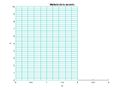
Seleccionar para ampliar

En física, las ecuaciones de Navier-Stokes son un conjunto de ecuaciones en derivadas parciales no lineales que describen el movimiento de un fluido viscoso. En este caso, la velocidad de las partículas del fluido viene dada por el campo vectorial [math]\overrightarrow{u}\left ( \rho ,\theta ,z \right )=f\left ( \rho \right )\overrightarrow{ez}[/math] y su presión [math]p\left ( x,y \right )=p1+\left ( p2-p1 \right )\left ( z-1 \right )[/math], donde [math]\mu[/math] es el coeficiente de viscosidad, p1 es la presión en los puntos z = 1, p2 la presión en los puntos z = 2.
Se utilizará la ecuación de Navier-Stoker estacionaria (independiente del tiempo), ya que [math]\left ( \overrightarrow{u},p \right )[/math] satisface dicha ecuación. Se va despreciar el primer término, la parte convectiva. [math]\left ( \overrightarrow{u}\cdot \bigtriangledown \right )\cdot u +\bigtriangledown p = \mu \Delta \overrightarrow{u}[/math].
Se comprueba que [math]f\left ( \rho \right )[/math] satisface la ecuación diferencial:
[math] \frac{1}{\rho } \frac{\partial }{\partial \rho } \left ( \rho \frac{\partial f(\rho )}{\partial \rho } \right ) = \frac{p_{2}-p_{1}}{\mu }[/math]
Se supone previamente que la velocidad del fluido en [math] \rho =2[/math] es nula y en [math] \rho =0[/math] no se hace infinito. Multiplicando por [math] \rho [/math] e integrando dos veces se obtiene:
[math]f\left ( \rho \right )=\frac{p2-p1}{4\mu}\rho ^{2} +Cln\left (\rho \right )+K[/math]
[math]f\left (2\right )=0[/math], [math]K=\frac{p1-p2}{\mu}[/math]
[math]f\left ( 0 \right )=0[/math],
[math]C=0[/math]
Entonces se obtiene:
[math]f\left ( \rho \right )=\frac{1}{\mu }\left [ \frac{p2-p1}{4 }\rho ^{2} +p1-p2\right ][/math]
Finalmente, se verificará que se cumple la condición de incompresibilidad (ya que el fluido siempre ocupa el mismo volumen). La divergencia del campo en un punto indica si una partícula de fluido sometida a la fuerza del campo se expande o se contrae, dependiendo del signo, o si el fluido es incompresible (siendo la divergencia cero, como es en este caso).
[math]\bigtriangledown \cdot \overrightarrow{u}=0=\frac{1}{\rho } \left\{ \frac{\partial }{\partial \rho }\left ( \rho u_{\rho } \right )+ \frac{\partial }{\partial \theta }(u_{\theta })+ \frac{\partial }{\partial z}(\rho u_{z})\right\}[/math]
4 Campo de presiones y el campo de velocidades
Para este apartado las variables p1,p2 y [math]\mu[/math] tomarán los siguientes valores: [math]p1=2, p2=1 ,\mu=1[/math]
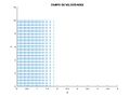
4.1 Campo de velocidades
Entonces la velocidad de las partículas del fluido viene dada por; [math]\overrightarrow{u}\left ( \rho ,\theta ,z \right )=\left ( \frac{-1}{4 }\rho ^{2} +1\right )\overrightarrow{ez}[/math]. En el siguiente gráfico se puede observar como la velocidad de las párticulas del fluido es inversamente proporcional al radio de la tubería, siendo máxima en el eje de la tubería y mínima o nula en las paredes o contorno de ella (Ley de Poiseuille).
x=0:0.2:2;
y=0:0.2:10;
[X,Y]=meshgrid(x,y);
ux=(-1./4).*xx.^2+1;
uy=0.*yy;
hold on
quiver(xx,yy,ux,uy)
axis([0,5,0,12])
xlabel('ρ');
ylabel('z');
hold off
view(2)
title('CAMPO DE VELOCIDADES')
Seleccionar para ampliar

4.2 Campo de presiones
Y la presión del fluido: [math]p\left ( x,y \right )=3-z[/math],dependiente única y exclusivamente de la altura z. En este gráfico se observa que al aumentar la altura, la presión dismuye, y viceversa.
x=0:0.2:2;
z=0:0.2:10;
[X,Z]=meshgrid(x,z);
figure(1);
p=3-Z;
surf(X,Z,p);
colorbar;
view(2);
axis([0,3,0,10]);
title('Campo de presiones');
xlabel('ρ');
ylabel('z');
Seleccionar para ampliar

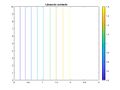
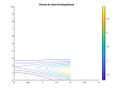
5 Líneas de corriente
Para dibujar las líneas de corriente del campo [math]\overrightarrow{u}[/math], es decir, las líneas que son tangenes a [math]\overrightarrow{u}[/math] en cad apunto, es necesario calcular el campo [math]\overrightarrow{v}[/math] que en cada punto es ortogonal a [math]\overrightarrow{u}[/math]. Siendo [math]\overrightarrow{v}=\overrightarrow{e_{\theta }}\times \overrightarrow{u}[/math]. El campo [math]\overrightarrow{v}[/math] es irrotacional por ser nula la divergencia de [math]\overrightarrow{u}[/math] y ,además, tiene un potencial escalar [math]\psi [/math],([math]\bigtriangledown \psi =\overrightarrow{v}[/math]), que se conoce como función de corriende de [math]\overrightarrow{u}[/math].
[math]\overrightarrow{v}=\begin{vmatrix} \overrightarrow{e_{\rho }} & \overrightarrow{e_{\theta }}&\overrightarrow{e_{z}} \\ 0&1 &0 \\ 0&0 &f\left ( \rho \right ) \end{vmatrix}=f\left ( \rho \right )\overrightarrow{e_{\rho }} \rightarrow \overrightarrow{v}=f\left ( \rho \right )\overrightarrow{e_{\rho }}[/math].
Sustituyendo [math]f\left ( \rho \right )[/math] se obtiene:
[math]\overrightarrow{v}=\left ( \frac{p2-p1}{4\mu }\rho ^{2} +\frac{p1-p2}{\mu }\right )\overrightarrow{e_{\rho }}[/math].
Para calcular [math]\psi [/math], obtenemos su gradiente e igualmaos al campo [math]\overrightarrow{v}[/math], [math]\bigtriangledown \psi =\overrightarrow{v}[/math].
[math]\bigtriangledown \psi=\frac{d\psi }{d\rho }\overrightarrow{e_{\rho }}+\frac{1}{\rho }\frac{d\psi }{d\theta }\overrightarrow{e_{\theta }}+\frac{d\psi }{dz}\overrightarrow{e_{z}}=\overrightarrow{v}[/math]. Por ende: [math]\frac{d\psi }{d\rho }=\frac{p2-p1}{4\mu }\rho ^{2} +\frac{p1-p2}{\mu }\ [/math].
Tras integrar nos queda finalmente que [math]\psi=\frac{p2-p1}{24\mu }\rho ^{2} +\frac{p1-p2}{\mu }\rho [/math].
Sustituyendo en la anterior función los valores asignados, el resultado de la función potencial será: [math] \psi= -\frac{1}{24} \rho ^{2} + \rho[/math]
En la siguiente imagen, con ayuda del programa informático Matlab, se representan las líneas [math]\psi=cte [/math]. Posteriormente se comprueba que , efectivamente, son líneas de corriente de [math]\overrightarrow{u}[/math]. Es decir, que son tangentes a dicho campo en cada punto. Siguen la dirección de [math]\overrightarrow{e_{z}}[/math] por lo que sigue el sentido de la tubería.
x=0:0.2:2;
y=0:0.2:10;
[X,Y]=meshgrid(x,y);
lineas=(-1./24).*X.^2+X;
contour(X,Y,lineas);
axis([0,3,0,10]);
colorbar
title('Líneas de corriente');
Seleccionar para ampliar

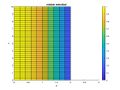
6 Comportamiento del módulo de la velocidad
Se observa en que puntos el módulo de la velocidad del fluido es máxima. En el siguiente gráfico se observa el comportamiento del módulo de la velocidad en función de [math]\rho[/math], es máximo en el eje de la tubería al igual que la velocidad.
x=0:0.2:2;
y=0:0.2:10;
[X,Y]=meshgrid(x,y);
z=(-1./4).*X.^2+1;
hold on
surf(X,Y,z)
colorbar
axis([0,3,0,10])
xlabel('ρ');
ylabel('z');
hold off
view(2)
title('módulo velocidad')
Seleccionar para ampliar

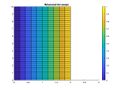
7 Rotacional
El rotacional de [math]\overrightarrow{u}[/math] se obtiene:
[math]\bigtriangledown\times\overrightarrow{u}\left ( \rho ,\theta ,z \right )= \frac{1}{\rho }\begin{vmatrix} \overrightarrow{e_{\rho }} &\rho \overrightarrow{e_{\theta }} & \overrightarrow{e_{z}}\\ \frac{d}{d\rho }& \frac{d}{d\theta } &\frac{d}{dz} \\ 0 & 0 &f\left ( \rho \right ) \end{vmatrix}=-f'\left ( \rho \right )\overrightarrow{e_{\theta }}[/math]
Tal que [math]f'\left ( \rho \right )=\frac{1}{2}\frac{p2-p1}{\mu }\rho[/math] , entonces el rotacional quedaría: [math]\bigtriangledown\times\overrightarrow{u}\left ( \rho ,\theta ,z \right )=-\frac{1}{2}\frac{p2-p1}{\mu }\rho \overrightarrow{e_{\theta }}[/math]
x=0:0.2:2;
y=0:0.2:10;
[xx,yy]=meshgrid(x,y);
rot=abs((1./2).*xx);
hold on
surf(xx,yy,rot);
colorbar;
view(2);
axis([0,3,0,10]);
title('Rotacional del campo');
hold off
Seleccionar para ampliar

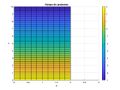
8 Campo de temperaturas
La temperatura a la que se encuentra sometido nuestro fluido viene dada por el siguiente campo escalar:
[math]T\left ( \rho , \theta ,z \right )= 1+ \left ( \rho -1/2 \right )^{2} \cdot e^{-\left ( z-1 \right )^{2}}[/math]
Conservando el sistema en coordenadas cilíndricas y usamos la fórmula del gradiente:
[math]\bigtriangledown T = \frac{df}{dz}\overrightarrow{e_{\rho }} + \frac{1}{\rho }\frac{df}{d\theta }\overrightarrow{e_{\theta }} + \frac{df}{dz}\overrightarrow{e_{z}}[/math]
Finalmente, después de realizar el cálculo del gradiente, expresamos el campo tal que: [math]\bigtriangledown T= \left ( 2\rho -1 \right )e^{-z^{2}+2z-1}\cdot \overrightarrow{e_{\rho }} + \left ( \rho ^{2}-\rho +\frac{1}{4} \right )\left ( -2z +2 \right )\cdot e^{-z^{2}+2z-1}\cdot \overrightarrow{e_{z}}[/math]
A continuación, se detalla el campo de temperaturas de forma gráfica y visual mediante el programa Matlab
8.1 Campo
x=0:0.2:2;
y=0:0.2:10;
[X,Y]=meshgrid(x,y);
rho=sqrt(X.^2+Y.^2);
hold on
T=1+((rho-(1/2)).^2).*(exp(-(Y-1).^2));
surf(X,Y,T);
view
axis([0,3,0,10]);
colorbar
title('Campo de temperaturas')
hold off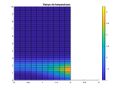
Seleccionar para ampliar

8.2 Curvas de nivel del campo
x=0:0.2:2;
y=0:0.2:10;
[X,Y]=meshgrid(x,y);
rho=sqrt(X.^2+Y.^2);
hold on
T=1+((rho-(1/2)).^2).*(exp(-(Y-1).^2));
contour(X,Y,T,10);
axis([0,3,0,10]);
view(2);
title('Curvas de nivel de temperatura')
colorbar
hold off
Seleccionar para aumentar

9 Gradiente de la temperatura
x=0:0.2:2;
y=0:0.2:10;
[X,Y]=meshgrid(x,y);
figure(1);
rho=sqrt(X.^2+Y.^2);
T=1+((rho-(1/2)).^2).*(exp(-(Y-1).^2));
[TX,TY]=gradient(T);
hold on
quiver(X,Y,TX,TY)
axis([0,3,0,10]);
title('Gradiente de temperatura');
shading flat
grid on
hold off

Seleccionar para aumentar

10 Caudal
Sea Q el caudal que atraviesa una sección de la tubería, [math]Q\left ( m^{3}/s \right )=\int_{S}^{}\overrightarrow{u}\overrightarrow{n}dS=\int_{S}^{}\left ( \frac{1}{4}\frac{p2-p1}{\mu }\rho ^{2}+\frac{p1-p2}{\mu }\rho \right )\overrightarrow{e_{z}}\cdot \overrightarrow{e_{z}} dS=\int_{0}^{2\Pi }\int_{0}^{2}\left ( \frac{1}{4}\frac{p2-p1}{\mu }\rho ^{2}+\frac{p1-p2}{\mu }\rho \right )d_{\rho }d_{\theta }=...=\frac{\Pi }{3}\left ( \frac{p2-p1}{\mu } \right )+4\Pi \frac{p1-p2}{\mu }[/math].
Tomando los siguientes valores: [math]p1=2, p2=1 ,\mu=1[/math], [math]Q=11.52\left ( m^{3}/s \right )[/math].