Diferencia entre revisiones de «Approximation of the heat equation: Fourier method»
(→MATLAB code) |
|||
| (No se muestran 14 ediciones intermedias del mismo usuario) | |||
| Línea 1: | Línea 1: | ||
| + | == Introduction == | ||
Let <math>{\bf u(x_1,x_2,x_3,t)}</math> be the temperature at the point <math>(x_1,x_2,x_3)\in </math> bar, and time <math>t>0</math>. | Let <math>{\bf u(x_1,x_2,x_3,t)}</math> be the temperature at the point <math>(x_1,x_2,x_3)\in </math> bar, and time <math>t>0</math>. | ||
| Línea 22: | Línea 23: | ||
We describe below the Fourier method to approximate the solutions of this system. | We describe below the Fourier method to approximate the solutions of this system. | ||
| + | |||
| + | == Fourier method == | ||
The main point is to observe that, if <math>\varphi(x)</math> is solution of the eigenvalue problem | The main point is to observe that, if <math>\varphi(x)</math> is solution of the eigenvalue problem | ||
| + | |||
<math> | <math> | ||
\left\{ \begin{array}{l} | \left\{ \begin{array}{l} | ||
| Línea 29: | Línea 33: | ||
\varphi(0)=0, \quad \varphi(L)=0, \end{array} \right. | \varphi(0)=0, \quad \varphi(L)=0, \end{array} \right. | ||
</math> | </math> | ||
| + | |||
for some <math>\lambda</math>, then | for some <math>\lambda</math>, then | ||
| + | |||
<math> | <math> | ||
u(x,t)=\varphi(x) e^{-\lambda t} | u(x,t)=\varphi(x) e^{-\lambda t} | ||
</math> | </math> | ||
| + | |||
is a solution of the heat equation <math>u_t-u_{xx}=0</math> and the boundary conditions <math>u(0,t)=u(L,t)=0.</math> | is a solution of the heat equation <math>u_t-u_{xx}=0</math> and the boundary conditions <math>u(0,t)=u(L,t)=0.</math> | ||
| + | The eigenvalues of the above eigenvalue problem are <math>\lambda_k=\frac{k^2 \pi^2}{L^2}</math> with <math>k=1,2,3,...</math> and the associated eigenfunctions are | ||
| + | |||
| + | <math> | ||
| + | \varphi_k=\sin(\frac{k\pi x}{L}). | ||
| + | </math> | ||
| + | |||
| + | Therefore, all these functions are solutions of the heat equation and boundary conditions | ||
| + | |||
| + | <math> | ||
| + | u_k (x,t)= e^{-k^2\pi^2 /L^2 t}\sin(\frac{k\pi x}{L}) | ||
| + | </math> | ||
| + | |||
| + | Thus, we only have to deal with the initial conditions. We consider two different cases: | ||
| + | |||
| + | ==The initial condition is a linear combination of eigenfunctions== | ||
| + | |||
| + | We assume that we can write the initial condition <math>u_0(x)</math> as | ||
| + | |||
| + | <math> | ||
| + | u^0(x)=\sum_{k=1}^N c_k \sin(\frac{k\pi x}{L}), | ||
| + | </math> | ||
| + | |||
| + | for some coefficients <math>c_k \in \mathbb{R}</math>. Then | ||
| + | |||
| + | <math> | ||
| + | u(x,t)=\sum_{k=1}^N c_k e^{-k^2\pi^2/L^2t} \sin(\frac{k\pi x}{L}), | ||
| + | </math> | ||
| + | |||
| + | is a solution of the full system: heat equation, boundary conditions and initial conditions. | ||
| + | |||
| + | '''Example''' | ||
| + | |||
| + | Consider the problem | ||
| + | |||
| + | <math> | ||
| + | \left\{ \begin{array}{lll} | ||
| + | u_t-u_{xx}=0, \;\; &x \in (0,1), \;\; t\in (0,3], \\ u(0, t)= 0, \hspace{0.3cm} u(1,t)=0, \;\; & t \in (0, 3], \\ u(x,0)= 2\sin(\pi x) -4\sin(3\pi x), \;\; & x \in [0,2], | ||
| + | \end{array} \right. | ||
| + | </math> | ||
| + | |||
| + | In this case <math>c_1=2</math> and <math>c_3=-4</math>. The solution is: | ||
| + | |||
| + | <math> | ||
| + | u(x,t)= 2 e^{-\pi^2 t} \sin(\pi x) -4 e^{-3^2\pi^2 t} \sin(3\pi x) , | ||
| + | </math> | ||
| + | |||
| + | == MATLAB code == | ||
| + | {{matlab|codigo= | ||
| + | % Draw solutions of heat equation | ||
| + | clear all | ||
| + | dx=1/100; % space mesh step | ||
| + | x=0:dx:1; %space mesh | ||
| + | dt=1/100; % time mesh step | ||
| + | t=0:dt:2; % time mesh | ||
| + | % Fourier coefficients of u0 | ||
| + | ck=[2, 0, -4]; | ||
| + | |||
| + | % meshgrid | ||
| + | [xx,tt]=meshgrid(x,t); | ||
| + | % first term: | ||
| + | u=ck(1)*exp(-pi^2*tt).*sin(pi*xx); | ||
| + | for k=2:length(ck) | ||
| + | % add the k-term | ||
| + | u=u+ck(k)*exp(-k^2*pi^2*tt).*sin(k*pi*xx); | ||
| + | end | ||
| + | figure(2) | ||
| + | surf(xx,tt,u) | ||
| + | }} | ||
| + | |||
| + | ==The initial condition is not a finite linear combination of eigenfunctions== | ||
| + | |||
| + | In this case, the main idea is to approximate the initial condition <math>u_0(x)</math> by | ||
| + | |||
| + | <math> | ||
| + | u^0(x) \sim \sum_{k=1}^N c_k \sin(\frac{k\pi x}{L}), | ||
| + | </math> | ||
| + | |||
| + | for some coefficients <math>c_k \in \mathbb{R}</math>. Then | ||
| + | |||
| + | <math> | ||
| + | u(x,t)\sim \sum_{k=1}^N c_k e^{-k^2\pi^2/L^2t} \sin(\frac{k\pi x}{L}), | ||
| + | </math> | ||
| + | |||
| + | is an approximated solution of the full system: heat equation, boundary conditions and initial conditions. | ||
| + | |||
| + | As we know, any <math>L^2(0,1)</math>-function can be approximated with a finite number of terms of the Fourier series and this allows to find approximations of heat solutions. | ||
| + | |||
| + | <gallery> | ||
| + | Eig4.jpg|Initial condition and approximation | ||
| + | Heat4.jpg|Approximate solution | ||
| + | </gallery> | ||
| + | |||
| + | ==Example: == | ||
| + | |||
| + | Consider the problem | ||
| + | |||
| + | <math> | ||
| + | \left\{ \begin{array}{lll} | ||
| + | u_t-u_{xx}=0, \;\; &x \in (0,2), \;\; t\in (0,3], \\ u(0, t)= 0, \hspace{0.3cm} u(2,t)=0, \;\; & t \in (0, 3], \\ u(x,0)= e^{-k(x-1)^2}, \;\; & x \in [0,2], | ||
| + | \end{array} \right. | ||
| + | </math> | ||
| + | |||
| + | We solve it by the Fourier method | ||
| + | |||
| + | '''Step 1:''' Solve the associated eigenvalue problem | ||
| + | |||
| + | The eigenvalue problem is | ||
| + | |||
| + | <math> | ||
| + | \left\{ \begin{array}{ll} | ||
| + | \varphi''+ \lambda \varphi =0, \hspace{0.4cm} x \in (0,2), \\ \varphi(0)=\varphi(2)=0. | ||
| + | \end{array} \right. | ||
| + | </math> | ||
| + | |||
| + | The eigenvalues and eigenfunctions are | ||
| + | |||
| + | <math> | ||
| + | \mu_k= \left( \frac{k\pi}{2} \right)^2 , \;\;\; \varphi_k(x)=\sin \frac{k \pi x}{2}, \;\; k=1,2, \cdot\cdot \cdot . | ||
| + | </math> | ||
| + | |||
| + | '''Step 2:''' Approximate the initial data by its projection on a finite dimensional subspace | ||
| + | |||
| + | Choose Q and take | ||
| + | |||
| + | <math> | ||
| + | e^{-k(x-1)^2} \approx \sum_{k=1}^{Q} {c_k} \sin \frac{k \pi x}{2}, | ||
| + | </math> | ||
| + | |||
| + | where | ||
| + | |||
| + | <math> | ||
| + | {c_k=\frac{\int_0^1 e^{-k(x-1)^2} \sin \frac{k \pi x}{2}dx}{\int_0^1 \sin^2 \frac{k \pi x}{2} dx}.} | ||
| + | </math> | ||
| + | |||
| + | '''Step 3:''' State the approximate problem for w | ||
| + | |||
| + | Approximate problem: | ||
| + | |||
| + | <math> | ||
| + | \left\{ \begin{array}{lll} | ||
| + | w_t-w_{xx}=0, \;\; & x \in (0,2), \;\; t\in (0,3], \\ w(0, t)= 0, \hspace{0.3cm} w(2,t)=0, \;\; &t \in (0, 3], \\ w(x,0)= \sum_{k=1}^{Q} {c_k} \sin \frac{k \pi x}{2}, \;\; & x \in [0,2], | ||
| + | \end{array} \right. | ||
| + | </math> | ||
| + | |||
| + | If we assume that the solution is of the form | ||
| + | |||
| + | <math> | ||
| + | w_Q(x,t)=\sum_{k=1}^{Q} {T_k(t)}\sin \frac{k \pi x}{2}, | ||
| + | </math> | ||
| + | |||
| + | then substituting in the heat equation we obtain an equation for each Fourier coefficient. | ||
| + | |||
| + | <math> | ||
| + | \left\{ \begin{array}{l} | ||
| + | T'_k(t) + \frac{k^2 \pi^2}{4} T_k(t)=0, \\ | ||
| + | T_k(0)={c_k}, \end{array} \right. | ||
| + | \;\; k=1,2, \cdot \cdot \cdot, Q. | ||
| + | </math> | ||
| + | |||
| + | The solution of this equation is: | ||
| + | |||
| + | <math> | ||
| + | T_k(t)=c_k e^{-\frac{k^2 \pi^2}{4} t}, \hspace{0.4cm} t \in [0,3], | ||
| + | </math> | ||
| + | |||
| + | and therefore | ||
| + | |||
| + | <math> | ||
| + | w_Q(x,t)=\sum_{k=1}^{Q} c_k e^{-\frac{k^2 \pi^2}{4} t}\sin \frac{k \pi x}{2}, | ||
| + | </math> | ||
| + | |||
| + | == MATLAB code == | ||
| + | {{matlab|codigo= | ||
| + | % Fourier series approximatin | ||
| + | clear all | ||
| + | % Interval | ||
| + | a=0; b=2; | ||
| + | % Define the initial data that we are going to approximate | ||
| + | u0=@(x) (1-2*abs(x-1)); | ||
| + | |||
| + | % Number of Fourier coefficients M | ||
| + | M=5; | ||
| + | |||
| + | % space discretization | ||
| + | N=100; dx=(b-a)/N; | ||
| + | x=a:dx:b; | ||
| + | |||
| + | % Compute the Fourier coefficients | ||
| + | aproxima=0; % aproximate function | ||
| + | for k=1:M | ||
| + | p=sin(k*pi*x/2); % eigenfunction | ||
| + | c(k)=trapz(x,u0(x).*p)/trapz(x,p.^2); | ||
| + | aproxima=aproxima+c(k)*p; | ||
| + | end | ||
| + | |||
| + | % Draw the function and the approximation | ||
| + | figure(1) | ||
| + | plot(x,[aproxima;u0(x)]) | ||
| + | |||
| + | % Draw solutions of heat equation | ||
| + | dt=1/100; % time mesh step | ||
| + | t=0:dt:2; % time mesh | ||
| + | |||
| + | [xx,tt]=meshgrid(x,t); | ||
| + | u=c(1)*exp(-pi^2/4*tt).*sin(pi*xx/2); | ||
| + | for k=2:M | ||
| + | u=u+c(k)*exp(-k^2*pi^2/4*tt).*sin(k*pi*xx/2); | ||
| + | end | ||
| + | figure(2) | ||
| + | surf(xx,tt,u) | ||
| + | }} | ||
[[Categoría:Grado en Ingeniería Civil y Territorial]] | [[Categoría:Grado en Ingeniería Civil y Territorial]] | ||
Revisión actual del 11:26 26 abr 2016
Contenido
1 Introduction
Let [math]{\bf u(x_1,x_2,x_3,t)}[/math] be the temperature at the point [math](x_1,x_2,x_3)\in [/math] bar, and time [math]t\gt0[/math].
Assume that the cross section is so small that we can consider the bar as an unidimensional object in the interval [math]x\in [0,L][/math], [math] u(x_1,x_2,x_3,t)=u(x_1,t)=u(x,t). [/math]
If we assume that the extreme are at zero temperature, the system of equations for u is given by [math] \left\{ \begin{array}{l} u_t-u_{xx}=0, \qquad x\in(0,L), \qquad t\gt0, \\ u(0,t)=0, \qquad t\gt0, \\ u(L,t)=0, \qquad t\gt0, \\ u(x,0)=u^0(x), \qquad x\in(0,L). \end{array} \right. [/math] where [math]u_0(x)[/math] is a function that describes the initial temperature of the bar.
We describe below the Fourier method to approximate the solutions of this system.
2 Fourier method
The main point is to observe that, if [math]\varphi(x)[/math] is solution of the eigenvalue problem
[math] \left\{ \begin{array}{l} \varphi''(x)+\lambda \varphi(x)=0, \\ \varphi(0)=0, \quad \varphi(L)=0, \end{array} \right. [/math]
for some [math]\lambda[/math], then
[math] u(x,t)=\varphi(x) e^{-\lambda t} [/math]
is a solution of the heat equation [math]u_t-u_{xx}=0[/math] and the boundary conditions [math]u(0,t)=u(L,t)=0.[/math]
The eigenvalues of the above eigenvalue problem are [math]\lambda_k=\frac{k^2 \pi^2}{L^2}[/math] with [math]k=1,2,3,...[/math] and the associated eigenfunctions are
[math] \varphi_k=\sin(\frac{k\pi x}{L}). [/math]
Therefore, all these functions are solutions of the heat equation and boundary conditions
[math] u_k (x,t)= e^{-k^2\pi^2 /L^2 t}\sin(\frac{k\pi x}{L}) [/math]
Thus, we only have to deal with the initial conditions. We consider two different cases:
3 The initial condition is a linear combination of eigenfunctions
We assume that we can write the initial condition [math]u_0(x)[/math] as
[math] u^0(x)=\sum_{k=1}^N c_k \sin(\frac{k\pi x}{L}), [/math]
for some coefficients [math]c_k \in \mathbb{R}[/math]. Then
[math] u(x,t)=\sum_{k=1}^N c_k e^{-k^2\pi^2/L^2t} \sin(\frac{k\pi x}{L}), [/math]
is a solution of the full system: heat equation, boundary conditions and initial conditions.
Example
Consider the problem
[math] \left\{ \begin{array}{lll} u_t-u_{xx}=0, \;\; &x \in (0,1), \;\; t\in (0,3], \\ u(0, t)= 0, \hspace{0.3cm} u(1,t)=0, \;\; & t \in (0, 3], \\ u(x,0)= 2\sin(\pi x) -4\sin(3\pi x), \;\; & x \in [0,2], \end{array} \right. [/math]
In this case [math]c_1=2[/math] and [math]c_3=-4[/math]. The solution is:
[math] u(x,t)= 2 e^{-\pi^2 t} \sin(\pi x) -4 e^{-3^2\pi^2 t} \sin(3\pi x) , [/math]
4 MATLAB code
% Draw solutions of heat equation
clear all
dx=1/100; % space mesh step
x=0:dx:1; %space mesh
dt=1/100; % time mesh step
t=0:dt:2; % time mesh
% Fourier coefficients of u0
ck=[2, 0, -4];

% meshgrid
[xx,tt]=meshgrid(x,t);
% first term:
u=ck(1)*exp(-pi^2*tt).*sin(pi*xx);
for k=2:length(ck)
    % add the k-term
   u=u+ck(k)*exp(-k^2*pi^2*tt).*sin(k*pi*xx);
end
figure(2)
surf(xx,tt,u)
5 The initial condition is not a finite linear combination of eigenfunctions
In this case, the main idea is to approximate the initial condition [math]u_0(x)[/math] by
[math] u^0(x) \sim \sum_{k=1}^N c_k \sin(\frac{k\pi x}{L}), [/math]
for some coefficients [math]c_k \in \mathbb{R}[/math]. Then
[math] u(x,t)\sim \sum_{k=1}^N c_k e^{-k^2\pi^2/L^2t} \sin(\frac{k\pi x}{L}), [/math]
is an approximated solution of the full system: heat equation, boundary conditions and initial conditions.
As we know, any [math]L^2(0,1)[/math]-function can be approximated with a finite number of terms of the Fourier series and this allows to find approximations of heat solutions.
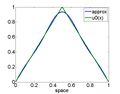
Initial condition and approximation
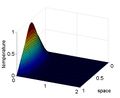
Approximate solution


6 Example:
Consider the problem
[math] \left\{ \begin{array}{lll} u_t-u_{xx}=0, \;\; &x \in (0,2), \;\; t\in (0,3], \\ u(0, t)= 0, \hspace{0.3cm} u(2,t)=0, \;\; & t \in (0, 3], \\ u(x,0)= e^{-k(x-1)^2}, \;\; & x \in [0,2], \end{array} \right. [/math]
We solve it by the Fourier method
Step 1: Solve the associated eigenvalue problem
The eigenvalue problem is
[math] \left\{ \begin{array}{ll} \varphi''+ \lambda \varphi =0, \hspace{0.4cm} x \in (0,2), \\ \varphi(0)=\varphi(2)=0. \end{array} \right. [/math]
The eigenvalues and eigenfunctions are
[math] \mu_k= \left( \frac{k\pi}{2} \right)^2 , \;\;\; \varphi_k(x)=\sin \frac{k \pi x}{2}, \;\; k=1,2, \cdot\cdot \cdot . [/math]
Step 2: Approximate the initial data by its projection on a finite dimensional subspace
Choose Q and take
[math] e^{-k(x-1)^2} \approx \sum_{k=1}^{Q} {c_k} \sin \frac{k \pi x}{2}, [/math]
where
[math] {c_k=\frac{\int_0^1 e^{-k(x-1)^2} \sin \frac{k \pi x}{2}dx}{\int_0^1 \sin^2 \frac{k \pi x}{2} dx}.} [/math]
Step 3: State the approximate problem for w
Approximate problem:
[math] \left\{ \begin{array}{lll} w_t-w_{xx}=0, \;\; & x \in (0,2), \;\; t\in (0,3], \\ w(0, t)= 0, \hspace{0.3cm} w(2,t)=0, \;\; &t \in (0, 3], \\ w(x,0)= \sum_{k=1}^{Q} {c_k} \sin \frac{k \pi x}{2}, \;\; & x \in [0,2], \end{array} \right. [/math]
If we assume that the solution is of the form
[math] w_Q(x,t)=\sum_{k=1}^{Q} {T_k(t)}\sin \frac{k \pi x}{2}, [/math]
then substituting in the heat equation we obtain an equation for each Fourier coefficient.
[math] \left\{ \begin{array}{l} T'_k(t) + \frac{k^2 \pi^2}{4} T_k(t)=0, \\ T_k(0)={c_k}, \end{array} \right. \;\; k=1,2, \cdot \cdot \cdot, Q. [/math]
The solution of this equation is:
[math] T_k(t)=c_k e^{-\frac{k^2 \pi^2}{4} t}, \hspace{0.4cm} t \in [0,3], [/math]
and therefore
[math] w_Q(x,t)=\sum_{k=1}^{Q} c_k e^{-\frac{k^2 \pi^2}{4} t}\sin \frac{k \pi x}{2}, [/math]
7 MATLAB code
% Fourier series approximatin
clear all
% Interval
a=0; b=2;
% Define the initial data that we are going to approximate
u0=@(x) (1-2*abs(x-1));

% Number of Fourier coefficients M
M=5;

% space discretization
N=100; dx=(b-a)/N;
x=a:dx:b;

% Compute the Fourier coefficients
aproxima=0;  % aproximate function
for k=1:M
   p=sin(k*pi*x/2); % eigenfunction
   c(k)=trapz(x,u0(x).*p)/trapz(x,p.^2);
   aproxima=aproxima+c(k)*p;
end

% Draw the function and the approximation
figure(1)
plot(x,[aproxima;u0(x)])

% Draw solutions of heat equation
dt=1/100; % time mesh step
t=0:dt:2; % time mesh

[xx,tt]=meshgrid(x,t);
u=c(1)*exp(-pi^2/4*tt).*sin(pi*xx/2);
for k=2:M
   u=u+c(k)*exp(-k^2*pi^2/4*tt).*sin(k*pi*xx/2);
end
figure(2)
surf(xx,tt,u)